Eigenvalue, eigenvector and eigenspace
From Wikipedia, the free encyclopedia

In mathematics, an eigenvector of a transformation[1] is a vector which, in the transformation, is multiplied by a constant factor, called the eigenvalue of that vector. (See Fig. 1). Often, a transformation is completely described by its eigenvalues and eigenvectors. The eigenspace for a factor is the set of eigenvectors with that factor as eigenvalue.
In the specific case of linear algebra, the eigenvalue problem is as follows. Given a matrix A, are there nonzero vectors x such that Ax is a multiple of x? If so, then the factor by which x is multiplied is called an eigenvalue of the matrix A, while x is called an eigenvector of A corresponding to this eigenvalue.
These concepts play a major role in several branches of both pure and applied mathematics — appearing prominently in linear algebra, functional analysis, and to a lesser extent in nonlinear situations.
It is common to prefix any natural name for the vector with eigen instead of saying eigenvector. For example, eigenfunction if the eigenvector is a function, eigenmode if the eigenvector is a harmonic mode, eigenstate if the eigenvector is a quantum state, and so on (e.g. the eigenface example below). Similarly for the eigenvalue, e.g. eigenfrequency if the eigenvalue is (or determines) a frequency.
[edit] History
Presently, eigenvalues are often introduced in the context of matrix theory. Historically, however, they arose in the study of quadratic forms and differential equations.
In the first half of the 18th century, Johann and Daniel Bernoulli, d'Alembert and Euler encountered eigenvalue problems when studying the motion of a rope, which they considered to be a weightless string loaded with a number of masses. Laplace and Lagrange continued their work in the second half of the century. They realized that the eigenvalues are related to the stability of the motion. They also used eigenvalue methods in their study of the solar system.[2]
Euler had also studied the rotational motion of a rigid body and discovered the importance of the principal axes. As Lagrange realized, the principal axes are the eigenvectors of the inertia matrix.[3] In the early 19th century, Cauchy saw how their work could be used to classify the quadric surfaces, and generalized it to arbitrary dimensions.[4] Cauchy also coined the term racine caractéristique (characteristic root) for what is now called eigenvalue; his term survives in characteristic equation.[5]
Fourier used the work of Laplace and Lagrange to solve the heat equation by separation of variables in his famous 1822 book Théorie analytique de la chaleur.[6] Sturm developed Fourier's ideas further and he brought them to the attention of Cauchy, who combined them with his own ideas and arrived at the fact that symmetric matrices have real eigenvalues.[4] This was extended by Hermite in 1855 to what are now called Hermitian matrices.[5] Around the same time, Brioschi proved that the eigenvalues of orthogonal matrices lie on the unit circle,[4] and Clebsch found the corresponding result for skew-symmetric matrices.[5] Finally, Weierstrass clarified an important aspect in the stability theory started by Laplace by realizing that defective matrices can cause instability.[4]
In the meantime, Liouville had studied similar eigenvalue problems as Sturm; the discipline that grew out of their work is now called Sturm-Liouville theory.[7] Schwarz studied the first eigenvalue of Laplace's equation on general domains towards the end of the 19th century, while Poincaré studied Poisson's equation a few years later.[8]
At the start of the 20th century, Hilbert studied the eigenvalues of integral operators by considering them to be infinite matrices.[9] He was the first to use the German word eigen to denote eigenvalues and eigenvectors in 1904, though he may have been following a related usage by Helmholtz. "Eigen" can be translated as "own", "peculiar to", "characteristic" or "individual"—emphasizing how important eigenvalues are to defining the unique nature of a specific transformation. For some time, the standard term in English was "proper value", but the more distinctive term "eigenvalue" is standard today.[10]
The first numerical algorithm for computing eigenvalues and eigenvectors appeared in 1929, when Von Mises published the power method. One of the most popular methods today, the QR algorithm, was proposed independently by Francis and Kublanovskaya in 1961.[11]
[edit] Definitions
- See also: Eigenplane
Linear transformations of space—such as rotation, reflection, stretching, compression, shear or any combination of these—may be visualized by the effect they produce on vectors. Vectors can be visualized as arrows pointing from one point to another.
- An eigenvector of a linear transformation is a vector that is either left unaffected or simply multiplied by a scale factor after the transformation (the former corresponds to a scale factor of 1).
- The eigenvalue of a non-zero eigenvector is the scale factor by which it has been multiplied.
- An eigenvalue of a linear transformation is a factor for which it has a non-zero eigenvector with that factor as its eigenvalue.
- The eigenspace corresponding to a given eigenvalue of a linear transformation is the vector space of all eigenvectors with that eigenvalue.
- The geometric multiplicity of an eigenvalue is the dimension of the associated eigenspace.
- The spectrum of a transformation on a finite dimensional vector space is the set of all its eigenvalues. (In the infinite-dimensional case, the concept of spectrum is more subtle and depends on the topology on the vector space.)
For instance, an eigenvector of a rotation in three dimensions is a vector located within the axis about which the rotation is performed. The corresponding eigenvalue is 1 and the corresponding eigenspace contains all the vectors along the axis. As this is a one-dimensional space, its geometric multiplicity is one. This is the only eigenvalue of the spectrum (of this rotation) that is a real number.
[edit] Examples
[edit] Mona Lisa
For the example shown on the right, the matrix that would produce a shear transformation similar to this would be.

The set of eigenvectors x for A is defined as those vectors which, when multiplied by A, result in a simple scaling λ of x. Thus, Ax = λx. The only effect of the matrix on these vectors will be to change their length, and possibly reverse their direction. So multiplying the right hand side by the Identity matrix I, we have Ax = (λI)x therefore

In order for this equation to have non trivial solutions, we require the determinant det(A − λI) which is called the characteristic polynomial of the matrix A to be zero. We can calculate the determinant as

and now we have obtained the characteristic polynomial (1 − λ)2 of the matrix A. There is in this case only one distinct solution of the equation (1 − λ)2 = 0, λ = 1. This is the eigenvalue of the matrix A.
Having found an eigenvalue, we can solve for the space of eigenvectors by finding the nullspace of A − (1)I. In other words by solving for vectors x which are solutions of

Substituting our obtained eigenvalue λ = 1,

Solving this new matrix equation, we find that vectors in the nullspace have the form

where c is an arbitrary constant. All vectors of this form, i.e. pointing straight up or down, are eigenvectors of the matrix A. The effect of applying the matrix A to these vectors is equivalent to multiplying them by their corresponding eigenvalue, in this case 1.
In general, 2-by-2 matrices will have two distinct eigenvalues, and thus two distinct eigenvectors. Whereas most vectors will have both their lengths and directions changed by the matrix, eigenvectors will only have their lengths changed, and will not change their direction, except perhaps to flip through the origin. Also, it is usually the case that the eigenvalue will be something other than 1, and so eigenvectors will be stretched, squashed and/or flipped through the origin by the matrix.
[edit] Other examples
As the Earth rotates, every arrow pointing outward from the center of the Earth also rotates, except those arrows which are parallel to the axis of rotation. Consider the transformation of the Earth after one hour of rotation: An arrow from the center of the Earth to the Geographic South Pole would be an eigenvector of this transformation, but an arrow from the center of the Earth to anywhere on the equator would not be an eigenvector. Since the arrow pointing at the pole is not stretched by the rotation of the Earth, its eigenvalue is 1.
Another example is provided by a rubber sheet expanding omnidirectionally about a fixed point in such a way that the distances from any point of the sheet to the fixed point are doubled. This expansion is a transformation with eigenvalue 2. Every vector from the fixed point to a point on the sheet is an eigenvector, and the eigenspace is the set of all these vectors.

However, three-dimensional geometric space is not the only vector space. For example, consider a stressed rope fixed at both ends, like the vibrating strings of a string instrument (Fig. 2). The distances of atoms of the vibrating rope from their positions when the rope is at rest can be seen as the components of a vector in a space with as many dimensions as there are atoms in the rope.
Assume the rope is a continuous medium. If one considers the equation for the acceleration at every point of the rope, its eigenvectors, or eigenfunctions, are the standing waves. The standing waves correspond to particular oscillations of the rope such that the acceleration of the rope is simply its shape scaled by a factor—this factor, the eigenvalue, turns out to be − ω2 where ω is the angular frequency of the oscillation. Each component of the vector associated with the rope is multiplied by a time-dependent factor sin(ωt). If damping is considered, the amplitude of this oscillation decreases until the rope stops oscillating, corresponding to a complex ω. One can then associate a lifetime with the imaginary part of ω, and relate the concept of an eigenvector to the concept of resonance. Without damping, the fact that the acceleration operator (assuming a uniform density) is Hermitian leads to several important properties, such as that the standing wave patterns are orthogonal functions.
[edit] Eigenvalue equation
Suppose T is a linear transformation of a finite-dimensional space, that is  for all scalars a, b, and vectors v, w. Then
  is an eigenvector and λ the corresponding eigenvalue of T if the equation:

is true, where T(vλ) is the vector obtained when applying the transformation T to vλ.
Consider a basis of the vector space that T acts on. Then T and vλ can be represented relative to that basis by a matrix AT—a two-dimensional array—and respectively a column vector vλ—a one-dimensional vertical array. The eigenvalue equation in its matrix representation is written

where the juxtaposition is matrix multiplication. Since, once a basis is fixed, T and its matrix representation AT are equivalent, we can often use the same symbol T for both the matrix representation and the transformation. This is equivalent to a set of n linear equations, where n is the number of basis vectors in the basis set. In this equation both the eigenvalue λ and the n components of vλ are unknowns.
However, it is sometimes unnatural or even impossible to write down the eigenvalue equation in a matrix form. This occurs for instance when the vector space is infinite dimensional, for example, in the case of the rope above. Depending on the nature of the transformation T and the space to which it applies, it can be advantageous to represent the eigenvalue equation as a set of differential equations. If T is a differential operator, the eigenvectors are commonly called eigenfunctions of the differential operator representing T. For example, differentiation itself is a linear transformation since
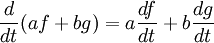
(f(t) and g(t) are differentiable functions, and a and b are constants).
Consider differentiation with respect to t. Its eigenfunctions h(t) obey the eigenvalue equation:
 ,
,
where λ is the eigenvalue associated with the function. Such a function of time is constant if λ = 0, grows proportionally to itself if λ is positive, and decays proportionally to itself if λ is negative. For example, an idealized population of rabbits breeds faster the more rabbits there are, and thus satisfies the equation with a positive lambda.
The solution to the eigenvalue equation is g(t) = exp(λt), the exponential function; thus that function is an eigenfunction of the differential operator d/dt with the eigenvalue λ. If λ is negative, we call the evolution of g an exponential decay; if it is positive, an exponential growth. The value of λ can be any complex number. The spectrum of d/dt is therefore the whole complex plane. In this example the vector space in which the operator d/dt acts is the space of the differentiable functions of one variable. This space has an infinite dimension (because it is not possible to express every differentiable function as a linear combination of a finite number of basis functions). However, the eigenspace associated with any given eigenvalue λ is one dimensional. It is the set of all functions g(t) = Aexp(λt), where A is an arbitrary constant, the initial population at t=0.
[edit] Spectral theorem
- For more details on this topic, see spectral theorem.
In its simplest version, the spectral theorem states that, under certain conditions, a linear transformation of a vector  can be expressed as a linear combination of the eigenvectors, in which the coefficient of each eigenvector is equal to the corresponding eigenvalue times the scalar product (or dot product) of the eigenvector with the vector . Mathematically, it can be written as:

where  and
and  stand for the eigenvectors and eigenvalues of
  . The simplest case in which the theorem is valid is the case where the linear transformation is given by a real symmetric matrix or complex Hermitian matrix; more generally the theorem holds for all normal matrices.
If one defines the nth power of a transformation as the result of applying it n times in succession, one can also define polynomials of transformations. A more general version of the theorem is that any polynomial P of is equal to:

The theorem can be extended to other functions of transformations like analytic functions, the most general case being Borel functions.
[edit] Eigenvalues and eigenvectors of matrices
[edit] Computing eigenvalues and eigenvectors of matrices
Suppose that we want to compute the eigenvalues of a given matrix. If the matrix is small, we can compute them symbolically using the characteristic polynomial. However, this is often impossible for larger matrices, in which case we must use a numerical method.
[edit] Symbolic computations
- For more details on this topic, see symbolic computation of matrix eigenvalues.
- Finding eigenvalues
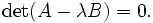
An important tool for describing eigenvalues of square matrices is the characteristic polynomial: saying that λ is an eigenvalue of A is equivalent to stating that the system of linear equations (A – λI) v = 0 (where I is the identity matrix) has a non-zero solution v (an eigenvector), and so it is equivalent to the determinant:

The function p(λ) = det(A – λI) is a polynomial in λ since determinants are defined as sums of products. This is the characteristic polynomial of A: the eigenvalues of a matrix are the zeros of its characteristic polynomial.
All the eigenvalues of a matrix A can be computed by solving the equation pA(λ) = 0. If A is an n×n matrix, then pA has degree n and A can therefore have at most n eigenvalues. If the matrix is over an algebraically closed field, such as the complex numbers, then the fundamental theorem of algebra says that the characteristic equation has exactly n roots (zeroes), counted with multiplicity. Therefore, any matrix over the complex numbers has an eigenvalue. All real polynomials of odd degree have a real number as a root, so for odd n, every real matrix has at least one real eigenvalue. However, if n is even, a matrix with real entries may not have any real eigenvalues. For any n, the non-real eigenvalues of a real matrix will come in conjugate pairs, just as the roots of a polynomial with real coefficients do.
- Finding eigenvectors
Once the eigenvalues λ are known, the eigenvectors can then be found by solving:

where v is in the null space of A − λI
An example of a matrix with no real eigenvalues is the 90-degree clockwise rotation:

whose characteristic polynomial is λ2 + 1 and so its eigenvalues are the pair of complex conjugates i, -i. The associated eigenvectors are also not real.
[edit] Numerical computations
- For more details on this topic, see eigenvalue algorithm.
In practice, eigenvalues of large matrices are not computed using the characteristic polynomial. Computing the polynomial becomes expensive in itself, and exact (symbolic) roots of a high-degree polynomial can be difficult to compute and express: the Abel–Ruffini theorem implies that the roots of high-degree (5 and above) polynomials cannot be expressed simply using nth roots. Effective numerical algorithms for approximating roots of polynomials exist, but small errors in the eigenvalues can lead to large errors in the eigenvectors. Therefore, general algorithms to find eigenvectors and eigenvalues, are iterative. The easiest method is the power method: a random vector v is chosen and a sequence of unit vectors is computed as
 ,
,  ,
,  , ...
, ...
This sequence will almost always converge to an eigenvector corresponding to the eigenvalue of greatest magnitude. This algorithm is easy, but not very useful by itself. However, popular methods such as the QR algorithm are based on it.
[edit] Properties
[edit] Algebraic multiplicity
The algebraic multiplicity of an eigenvalue λ of A is the order of λ as a zero of the characteristic polynomial of A; in other words, if λ is one root of the polynomial, it is the number of factors (t − λ) in the characteristic polynomial after factorization. An n×n matrix has n eigenvalues, counted according to their algebraic multiplicity, because its characteristic polynomial has degree n.
An eigenvalue of algebraic multiplicity 1 is called a "simple eigenvalue".
In an article on matrix theory, a statement like the one below might be encountered:
- "the eigenvalues of a matrix A are 4,4,3,3,3,2,2,1,"
meaning that the algebraic multiplicity of 4 is two, of 3 is three, of 2 is two and of 1 is one. This style is used because algebraic multiplicity is the key to many mathematical proofs in matrix theory.
Recall that above we defined the geometric multiplicity of an eigenvector to be the dimension of the associated eigenspace, the nullspace of λI − A. The algebraic multiplicity can also be thought of as a dimension: it is the dimension of the associated generalized eigenspace (1st sense), which is the nullspace of the matrix (λI − A)k for any sufficiently large k. That is, it is the space of generalized eigenvectors (1st sense), where a generalized eigenvector is any vector which eventually becomes 0 if λI − A is applied to it enough times successively. Any eigenvector is a generalized eigenvector, and so each eigenspace is contained in the associated generalized eigenspace. This provides an easy proof that the geometric multiplicity is always less than or equal to the algebraic multiplicity. The first sense should not to be confused with generalized eigenvalue problem as stated below.
For example:

It has only one eigenvalue, namely λ = 1. The characteristic polynomial is (λ − 1)2, so this eigenvalue has algebraic multiplicity 2. However, the associated eigenspace is the axis usually called the x axis, spanned by the unit vector  , so the geometric multiplicity is only 1.
Generalized eigenvectors can be used to calculate the Jordan normal form of a matrix (see discussion below). The fact that Jordan blocks in general are not diagonal but nilpotent is directly related to the distinction between eigenvectors and generalized eigenvectors.
[edit] Decomposition theorems for general matrices
The decomposition theorem is a version of the spectral theorem in the particular case of matrices. This theorem is usually introduced in terms of coordinate transformation. If U is an invertible matrix, it can be seen as a transformation from one coordinate system to another, with the columns of U being the components of the new basis vectors within the old basis set. In this new system the coordinates of the vector v are labeled v'. The latter are obtained from the coordinates v in the original coordinate system by the relation v' = Uv and, the other way around, we have v = U − 1v'. Applying successively v' = Uv, w' = Uw and U − 1U = I, to the relation Av = w defining the matrix multiplication provides A'v' = w' with A' = UAU − 1, the representation of A in the new basis. In this situation, the matrices A and A' are said to be similar.
The decomposition theorem states that, if one chooses as columns of U − 1 n linearly independent eigenvectors of A, the new matrix A' = UAU − 1 is diagonal and its diagonal elements are the eigenvalues of A. If this is possible the matrix A is diagonalizable. An example of non-diagonalizable matrix is given by the matrix A above. There are several generalizations of this decomposition which can cope with the non-diagonalizable case, suited for different purposes:
- the Schur triangular form states that any matrix is unitarily equivalent to an upper triangular one;
- the singular value decomposition, A = UΣV * where Σ is diagonal with U and V unitary matrices. The diagonal entries of A = UΣV * are nonnegative; they are called the singular values of A. This can be done for non-square matrices as well;
- the Jordan normal form, where A = XΛX − 1 where Λ is not diagonal but block-diagonal. The number and the sizes of the Jordan blocks are dictated by the geometric and algebraic multiplicities of the eigenvalues. The Jordan decomposition is a fundamental result. One might glean from it immediately that a square matrix is described completely by its eigenvalues, including multiplicity, up to similarity. This shows mathematically the important role played by eigenvalues in the study of matrices;
- as an immediate consequence of Jordan decomposition, any matrix A can be written uniquely as A = S + N where S is diagonalizable, N is nilpotent (i.e., such that Nq=0 for some q), and S commutes with N (SN=NS).
[edit] Some other properties of eigenvalues
The spectrum is invariant under similarity transformations: the matrices A and P-1AP have the same eigenvalues for any matrix A and any invertible matrix P. The spectrum is also invariant under transposition: the matrices A and AT have the same eigenvalues.
Since a linear transformation on finite dimensional spaces is bijective if and only if it is injective, a matrix is invertible if and only if zero is not an eigenvalue of the matrix.
Some more consequences of the Jordan decomposition are as follows:
- a matrix is diagonalizable if and only if the algebraic and geometric multiplicities coincide for all its eigenvalues. In particular, an n×n matrix which has n different eigenvalues is always diagonalizable; Under the same reasoning a matrix A with eigenvectors stored in matrix P will result in P-1⋅A⋅P=Σ where Σ is a diagonal matrix with the eigenvalues of A along the diagonal.
- the vector space on which the matrix acts can be viewed as a direct sum of its invariant subspaces span by its generalized eigenvectors. Each block on the diagonal corresponds to a subspace in the direct sum. When a block is diagonal, its invariant subspace is an eigenspace. Otherwise it is a generalized eigenspace, defined above;
- Since the trace, or the sum of the elements on the main diagonal of a matrix, is preserved by unitary equivalence, the Jordan normal form tells us that it is equal to the sum of the eigenvalues;
- Similarly, because the eigenvalues of a triangular matrix are the entries on the main diagonal, the determinant equals the product of the eigenvalues (counted according to algebraic multiplicity).
The location of the spectrum for a few subclasses of normal matrices are:
- All eigenvalues of a Hermitian matrix (A = A*) are real. Furthermore, all eigenvalues of a positive-definite matrix (v*Av > 0 for all non-zero vectors v) are positive;
- All eigenvalues of a skew-Hermitian matrix (A = −A*) are purely imaginary;
- All eigenvalues of a unitary matrix (A-1 = A*) have absolute value one;
Suppose that A is an m×n matrix, with m ≤ n, and that B is an n×m matrix. Then BA has the same eigenvalues as AB plus n − m eigenvalues equal to zero.
Each matrix can be assigned an operator norm, which depends on the norm of its domain. The operator norm of a square matrix is an upper bound for the moduli of its eigenvalues, and thus also for its spectral radius. This norm is directly related to the power method for calculating the eigenvalue of largest modulus given above. For normal matrices, the operator norm induced by the Euclidean norm is the largest moduli among its eigenvalues.
[edit] Conjugate eigenvector
A conjugate eigenvector or coneigenvector is a vector sent after transformation to a scalar multiple of its conjugate, where the scalar is called the conjugate eigenvalue or coneigenvalue of the linear transformation. The coneigenvectors and coneigenvalues represent essentially the same information and meaning as the regular eigenvectors and eigenvalues, but arise when an alternative coordinate system is used. The corresponding equation is

For example, in coherent electromagnetic scattering theory, the linear transformation A represents the action performed by the scattering object, and the eigenvectors represent polarization states of the electromagnetic wave. In optics, the coordinate system is defined from the wave's viewpoint, known as the Forward Scattering Alignment (FSA), and gives rise to a regular eigenvalue equation, whereas in radar, the coordinate system is defined from the radar's viewpoint, known as the Back Scattering Alignment (BSA), and gives rise to a coneigenvalue equation.
[edit] Generalized eigenvalue problem
A generalized eigenvalue problem (2nd sense) is of the form

where A and B are matrices. The generalized eigenvalues (2nd sense) λ can be obtained by solving the equation
The set of matrices of the form A − λB, where λ is a complex number, is called a pencil. If B is invertible, then the original problem can be written in the form

which is a standard eigenvalue problem. However, in most situations it is preferable not to perform the inversion, but rather to solve the generalized eigenvalue problem as stated originally.
An example is provided by the molecular orbital application below.
[edit] Entries from a ring
In the case of a square matrix A with entries in a ring, λ is called a right eigenvalue if there exists a nonzero column vector x such that Ax=λx, or a left eigenvalue if there exists a nonzero row vector y such that yA=yλ. The vectors x and y are the right and left eigenvectors of A.
If the ring is commutative, the left eigenvalues are equal to the right eigenvalues and are just called eigenvalues. If not, for instance if the ring is the set of quaternions, they may be different.
[edit] Infinite-dimensional spaces

If the vector space is an infinite dimensional Banach space, the notion of eigenvalues can be generalized to the concept of spectrum. The spectrum is the set of scalars λ for which  is not defined; that is, such that T − λ has no bounded inverse.
Clearly if λ is an eigenvalue of T, λ is in the spectrum of T. In general, the converse is not true. There are operators on Hilbert or Banach spaces which have no eigenvectors at all. This can be seen in the following example. The bilateral shift on the Hilbert space  (the space of all sequences of scalars
  such that
  converges) has no eigenvalue but has spectral values.
In infinite-dimensional spaces, the spectrum of a bounded operator is always nonempty. This is also true for an unbounded self adjoint operator. Via its spectral measures, the spectrum of any self adjoint operator, bounded or otherwise, can be decomposed into absolutely continuous, pure point, and singular parts. (See Decomposition of spectrum.)
The exponential growth or decay provides an example of a continuous spectrum, as does the vibrating string example illustrated above. The hydrogen atom is an example where both types of spectra appear. The bound states of the hydrogen atom correspond to the discrete part of the spectrum while the ionization processes are described by the continuous part. Fig. 3 exemplifies this concept in the case of the Chlorine atom.
[edit] Applications
[edit] Schrödinger equation

An example of an eigenvalue equation where the transformation is represented in terms of a differential operator is the time-independent Schrödinger equation in quantum mechanics:

where H, the Hamiltonian, is a second-order differential operator and ΨE, the wavefunction, is one of its eigenfunctions corresponding to the eigenvalue E, interpreted as its energy.
However, in the case where one is interested only in the bound state solutions of the Schrödinger equation, one looks for ΨE within the space of square integrable functions. Since this space is a Hilbert space with a well-defined scalar product, one can introduce a basis set in which ΨE and H can be represented as a one-dimensional array and a matrix respectively. This allows one to represent the Schrödinger equation in a matrix form. (Fig. 4 presents the lowest eigenfunctions of the Hydrogen atom Hamiltonian.)
The Dirac notation is often used in this context. A vector, which represents a state of the system, in the Hilbert space of square integrable functions is represented by  . In this notation, the Schrödinger equation is:

where is an eigenstate of H. It is a self adjoint operator, the infinite dimensional analog of Hermitian matrices (see Observable). As in the matrix case, in the equation above  is understood to be the vector obtained by application of the transformation H to .
[edit] Molecular orbitals
In quantum mechanics, and in particular in atomic and molecular physics, within the Hartree-Fock theory, the atomic and molecular orbitals can be defined by the eigenvectors of the Fock operator. The corresponding eigenvalues are interpreted as ionization potentials via Koopmans' theorem. In this case, the term eigenvector is used in a somewhat more general meaning, since the Fock operator is explicitly dependent on the orbitals and their eigenvalues. If one wants to underline this aspect one speaks of implicit eigenvalue equation. Such equations are usually solved by an iteration procedure, called in this case self-consistent field method. In quantum chemistry, one often represents the Hartree-Fock equation in a non-orthogonal basis set. This particular representation is a generalized eigenvalue problem called Roothaan equations.
[edit] Factor analysis
In Factor Analysis, the eigenvectors of a covariance matrix correspond to factors, and eigenvalues to factor loadings. Factor analysis is a statistical technique used in the social sciences and in marketing, product management, operations research, and other applied sciences that deal with large quantities of data. The objective is to explain most of the covariability among a number of observable random variables in terms of a smaller number of unobservable latent variables called factors. The observable random variables are modeled as linear combinations of the factors, plus unique variance terms.

[edit] Eigenfaces
In image processing, processed images of faces can be seen as vectors whose components are the brightnesses of each pixel. The dimension of this vector space is the number of pixels. The eigenvectors of the covariance matrix associated to a large set of normalized pictures of faces are called eigenfaces. They are very useful for expressing any face image as a linear combination of some of them. In the facial recognition branch of biometrics, eigenfaces provide a means of applying data compression to faces for identification purposes. Research related to eigen vision systems determining hand gestures has also been made. More on determining sign language letters using eigen systems can be found here: http://www.geigel.com/signlanguage/index.php
[edit] Tensor of inertia
In mechanics, the eigenvectors of the inertia tensor define the principal axes of a rigid body. The tensor of inertia is a key quantity required in order to determine the rotation of a rigid body around its center of mass.
[edit] Stress tensor
In solid mechanics, the stress tensor is symmetric and so can be decomposed into a diagonal tensor with the eigenvalues on the diagonal and eigenvectors as a basis. Because it is diagonal, in this orientation, the stress tensor has no shear components; the components it does have are the principal components.
[edit] Eigenvalues of a graph
In spectral graph theory, an eigenvalue of a graph is defined as an eigenvalue of the graph's adjacency matrix A, or (increasingly) of the graph's Laplacian matrix, which is either T−A or I − T − 1 / 2AT − 1 / 2, where T is a diagonal matrix holding the degree of each vertex, and in T − 1 / 2, 0 is substituted for 0 − 1 / 2.
The principal eigenvector of a graph is used to measure the centrality of its vertices. An example is Google's PageRank algorithm. The principal eigenvector of a modified adjacency matrix of the www-graph gives the page ranks as its components. The two eigenvectors with largest positive eigenvalues can also be used as x- and y-coordinates of vertices in drawing the graph via spectral layout methods. The second eigenvector can be used to partition the graph into clusters, via spectral clustering.
[edit] Notes
- ^ In this context, only linear transformations from a vector space to itself are considered.
- ^ See Hawkins (1975), §2; Kline (1972), pp. 807+808.
- ^ See Hawkins (1975), §2.
- ^ a b c d See Hawkins (1975), §3.
- ^ a b c See Kline (1972), pp. 807+808.
- ^ See Kline (1972), p. 673.
- ^ See Kline (1972), pp. 715+716.
- ^ See Kline (1972), pp. 706+707.
- ^ See Kline (1972), p. 1063.
- ^ See Aldrich (2006).
- ^ See Golub and Van Loan (1996), §7.3; Meyer (2000), §7.3.
- ^ T. W Gorczyca, Auger Decay of the Photoexcited Inner Shell Rydberg Series in Neon, Chlorine, and Argon, Abstracts of the 18th International Conference on X-ray and Inner-Shell Processes, Chicago, August 23-27 (1999).
[edit] References
- Abdi, H. "[1] (2007). Eigen-decomposition: eigenvalues and eigenvecteurs.In N.J. Salkind (Ed.): Encyclopedia of Measurement and Statistics. Thousand Oaks (CA): Sage.".
- John Aldrich, Eigenvalue, eigenfunction, eigenvector, and related terms. In Jeff Miller (Editor), Earliest Known Uses of Some of the Words of Mathematics, last updated 7 August 2006, accessed 22 August 2006.
- Claude Cohen-Tannoudji, Quantum Mechanics, Wiley (1977). ISBN 0-471-16432-1. (Chapter II. The mathematical tools of quantum mechanics.)
- John B. Fraleigh and Raymond A. Beauregard, Linear Algebra (3rd edition), Addison-Wesley Publishing Company (1995). ISBN 0-201-83999-7 (international edition).
- Gene H. Golub and Charles F. van Loan, Matrix Computations (3rd edition), Johns Hopkins University Press, Baltimore, 1996. ISBN 978-0-8018-5414-9.
- T. Hawkins, Cauchy and the spectral theory of matrices, Historia Mathematica, vol. 2, pp. 1–29, 1975.
- Roger A. Horn and Charles R. Johnson, Matrix Analysis, Cambridge University Press, 1985. ISBN 0-521-30586-1 (hardback), ISBN 0-521-38632-2 (paperback).
- Morris Kline, Mathematical thought from ancient to modern times, Oxford University Press, 1972. ISBN 0-19-501496-0.
- Carl D. Meyer, Matrix Analysis and Applied Linear Algebra, Society for Industrial and Applied Mathematics (SIAM), Philadelphia, 2000. ISBN 978-0-89871-454-8.
- Valentin, D.,Abdi, H, Edelman, B., O'Toole A.. "[2] (1997). Principal Component and Neural Network Analyses of Face Images: What Can Be Generalized in Gender Classification? Journal of Mathematical Psychology, 41, 398-412.".
[edit] External links
- ARPACK is a collection of FORTRAN subroutines for solving large scale (sparse) eigenproblems.
- IRBLEIGS, has MATLAB code with similar capabilities to ARPACK. (See this paper for a comparison between IRBLEIGS and ARPACK.)
- LAPACK is a collection of FORTRAN subroutines for solving dense linear algebra problems
- ALGLIB includes a partial port of the LAPACK to C++, C#, Delphi, etc.
- Eigenvalue (of a matrix) on PlanetMath
- MathWorld: Eigenvector
- Online calculator for Eigenvalues and Eigenvectors
- Online Matrix Calculator Calculates eigenvalues, eigenvectors and other decompositions of matrices online
- Vanderplaats Research and Development - Provides the SMS eigenvalue solver for Structural Finite Element. The solver is in the GENESIS program as well as other commercial programs. SMS can be easily use with MSC.Nastran or NX/Nastran via DMAPs.
- Videos of MIT Linear Algebra Course, spring 2005 - See Lecture Eigenvalues and Eigenvectors
- What are Eigen Values? from PhysLink.com's "Ask the Experts"
- Templates for the Solution of Algebraic Eigenvalue Problems Edited by Zhaojun Bai, James Demmel, Jack Dongarra, Axel Ruhe, and Henk van der Vorst (a guide to the numerical solution of eigenvalue problems)
'만들기 / Programming > research' 카테고리의 다른 글
| Color histogram (0) | 2007.07.31 |
|---|---|
| BRDF (0) | 2007.06.28 |
| K-nearest neighbor algorithm (1) | 2007.04.10 |
| Support vector machine (0) | 2007.04.05 |
| Principal components analysis (0) | 2007.04.04 |